This second part of this article deals with specific aspects that are helpful in the practical application of FFT measurements. FFT measurements are used in numerous applications. The results are usually presented as graphs and are easy to interpret. For accurate FFT measurements, there are some things to look out for. This article provides valuable tips.
As explained in the first part, the sampling rate fs of the measuring system and the block length BL are the two central parameters of an FFT. The sampling rate indicates how often the analog signal to be analyzed is scanned. When recording wav files via a commercially-available PC sound card, for example, the audio signal is usually sampled 44,100 times per second.
Nyquist Theorem
Harry Nyquist was the discoverer of a fundamental rule in the sampling of analog signals: the sampling frequency must be at least double the highest frequency of the signal. If, for example, a signal containing frequencies up to 24 kHz is to be sampled, a sampling rate of at least 48 kHz is required for this purpose. Half the sampling rate, in this example 24 kHz, is called the "Nyquist frequency".
But what happens if signals above the Nyquist frequency are fed in to the system?
Aliasing
For the most, a signal is sampled with a more-than-sufficient number of samples. With a 48 kHz sampling rate, for example, the 6 kHz frequency is sampled 8 times per cycle, while the 12 kHz frequency is only sampled 4 times per cycle. At the Nyquist frequency, only 2 samples are available per cycle.
With 2 samples or more it is still possible to reconstruct the signal without loss. If, however, less than 2 samples are available, artifacts which do not occur in the sampled (original) signal are generated.
Mirror frequencies
In the FFT, these artifacts appear as mirror frequencies. If the Nyquist frequency is exceeded, the signal is reflected at this imaginary limit and falls back into the useful frequency band. The following video shows an FFT system with 44.1 kHz sampling rate. A sweep signal of 15 kHz to 25 kHz is fed in to this system.
These unwanted mirror frequencies are counteracted with an analog low-pass filter (anti-aliasing filter) before the scanning. The filter ensures that frequencies above the Nyquist frequency are suppressed.
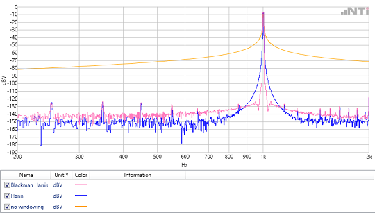
Time window
In the case of periodically-continuous signals, the time windowing serves to smooth the undesired transitional jumps at the end of the scanning (see part 1). This prevents smearing in the spectrum. There are numerous types of windows, some of which differ only slightly. When selecting the time window, the following rule applies: Each window requires a compromise between frequency selectivity and amplitude accuracy.
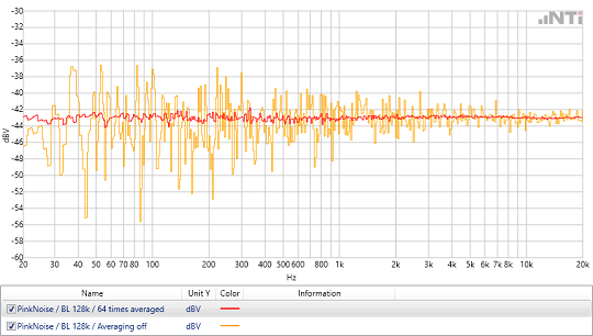
Averaging of Spectra
In the analysis of non-periodic signals, e.g. noise or music, it is often advantageous to capture multiple FFT blocks and determine mean values therefrom. There are two possible approaches:
- The classical mean: A number of FFTs are measured. Each result is considered in equal parts in the averaged final result. This method is suitable for measurements with a defined duration.
- The exponential mean: FFTs are continuously measured. Here, too, a fixed number of results of the continuous measurements are considered. However, the weighting is inversely proportional to the 'age' of the result. The oldest of the measurements is taken the least into account, the most recent measurement contributes most effectively to the averaged result. This exponential average is used when the spectrum is continuously monitored over a long period of time.
Power vs. Peak detector
Modern high-resolution FFT analyzers offer the possibility to decouple the number of measurement results from the FFT block length. This results in an increase in measurement performance time, especially for high-resolution FFTs. Thus, for example, with a 2MB block length it is no longer necessary to measure and represent more than 1 Million points (bins), but only the number necessary for the display, e.g. 1024.
The value chosen for each FFT bin can be defined in two ways:
- "MaxPeak": Here the maximum value of the FFT results is used. This type is well suited for the visual representation of FFTs
- "Power": Here the FFT results are summed up and averaged energetically. This is necessary when the FFT is used for calculations.
Calculations with FFT results
FFTs are mainly used to visualize signals. However, there are also applications where FFT results are used in calculations. For example, very simple levels of defined frequency bands can be calculated by adding them via an RSS (Root Sum Square) algorithm.
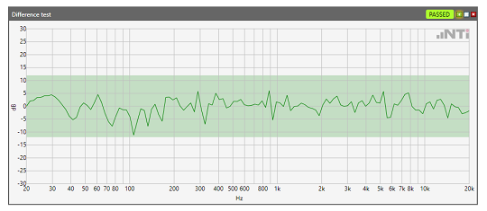
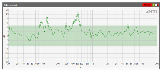
Another application is the comparison of spectra. The example below shows an acoustic measurement of a cordless screwdriver. The measured spectrum is subtracted from a defined reference spectrum. This difference is compared against an upper and lower tolerance. The upper spectrum shows a functional cordless screwdriver. In the lower, the acoustic spectrum suggests that the test specimen is defective.
Read more about the test solutions measuring FFT
FX100 オーディオアナライザ XL2 オーディオ&アコースティックアナライザ